A short introduction to Dask for Pandas developers

Dask is a useful framework for parallel processing in Python. If you already have some knowledge of Pandas or a similar data processing library, then this short introduction to Dask fundamentals is for you.

Specifically, we'll focus on some of the lower level Dask APIs. Understanding these is crucial to understanding common errors and performance issues you'll encounter when using the high-level APIs of Dask.

For normal use, you'll almost always use the higher level APIs directly, such as DaskDataFrame and DaskArray. This guide doesn’t aim to replace the official documentation but to supplement it.

You should at least take a short look at the following pages from the Dask Docs first:

• Overview of user interfaces;
• Dask graphs.

Setting up

To follow along, you should have Dask installed and a notebook environment like Jupyter Notebook running.

• Instructions for installing Dask.
• Instructions for installing Jupyter.

User interfaces in Dask

We'll start with a short overview of the high-level interfaces. These are similar to data frames from Pandas, so we’ll use them as a starting point to understand the low-level interfaces.

Creating and using dataframes with Dask

Let’s begin by creating a Dask dataframe. Run the following code in your notebook:

from pprint import pprint

import dask
import dask.dataframe as dd
import numpy as np

ddf = dask.datasets.timeseries(partition_freq="6d")
ddf

This looks similar to a Pandas dataframe, but there are no values in the table. You can see the type of each value in the first row, but the values themselves haven’t been computed yet.

This brings us to the first aspect of Dask that’s important to understand: computations are executed lazily. You created the definition of the computation, but it hasn’t actually been executed yet.

Notice how the variable is called ddf. This stands for dask dataframe. It's a useful convention to use this instead of df – common when dealing with Pandas dataframes – so you can easily distinguish them.

Understanding lazy computing

In general, you'll see lazy computing applied whenever you call a method on a Dask collection. Computation is not triggered at the time you call the method. Instead, on calling the method, the collection internally stores how to compute the results. Dask can decide later on the best place to run the actual computation.

Triggering computations on a Dask Dataframe

Now let's look at how we can tell Dask to trigger the computation. Run the following in a new cell in your notebook:

df = ddf.compute()
df

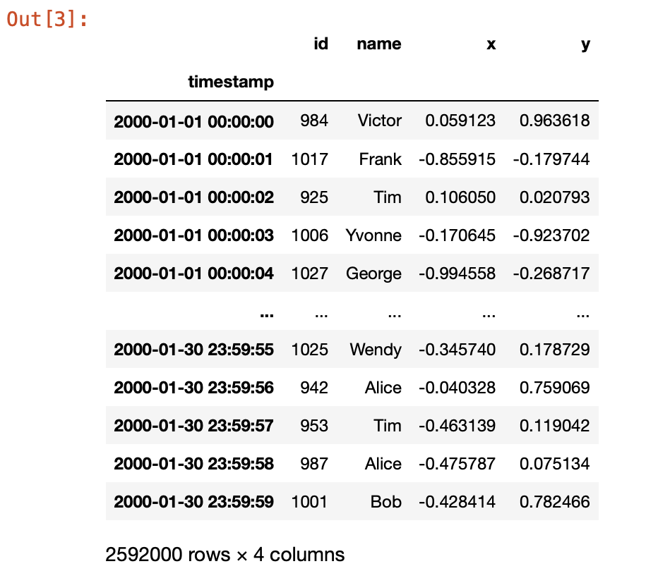
As you can see, the .compute() method triggers execution and we get a Pandas dataframe:

type(df)
# >>> pandas.core.frame.DataFrame

Computing simple operations on lazy dataframes

Next, let’s do a simple operation on our Dask dataframe, just to demonstrate laziness. We'll take each value of column x to the power of 2, first using a Dask dataframe and then a standard Pandas dataframe. We'll track the computation on each to compare.

from datetime import datetime

# Set up a bigger example random timeseries
ddf = dask.datasets.timeseries(start="2000-01-01", end="2003-01-01")

# Create the Pandas dataframe
df = ddf.compute()

# Time raising everything to the power of 2 using Dask
t1 = datetime.now()
a =  ddf.assign(x=ddf.x**2)
print(datetime.now() - t1)

# Time the same using Pandas
t1 = datetime.now()
b = df.assign(x=df.x**2)
print(datetime.now() - t1)

You should see output similar to the following:

0:00:00.004408
0:00:05.189730

The assign operation in Dask completed in 0.00 seconds, while it took just over 5 seconds with Pandas. If we examine the outputs, we'll see that Dask hasn't actually computed the values yet, while Pandas has.

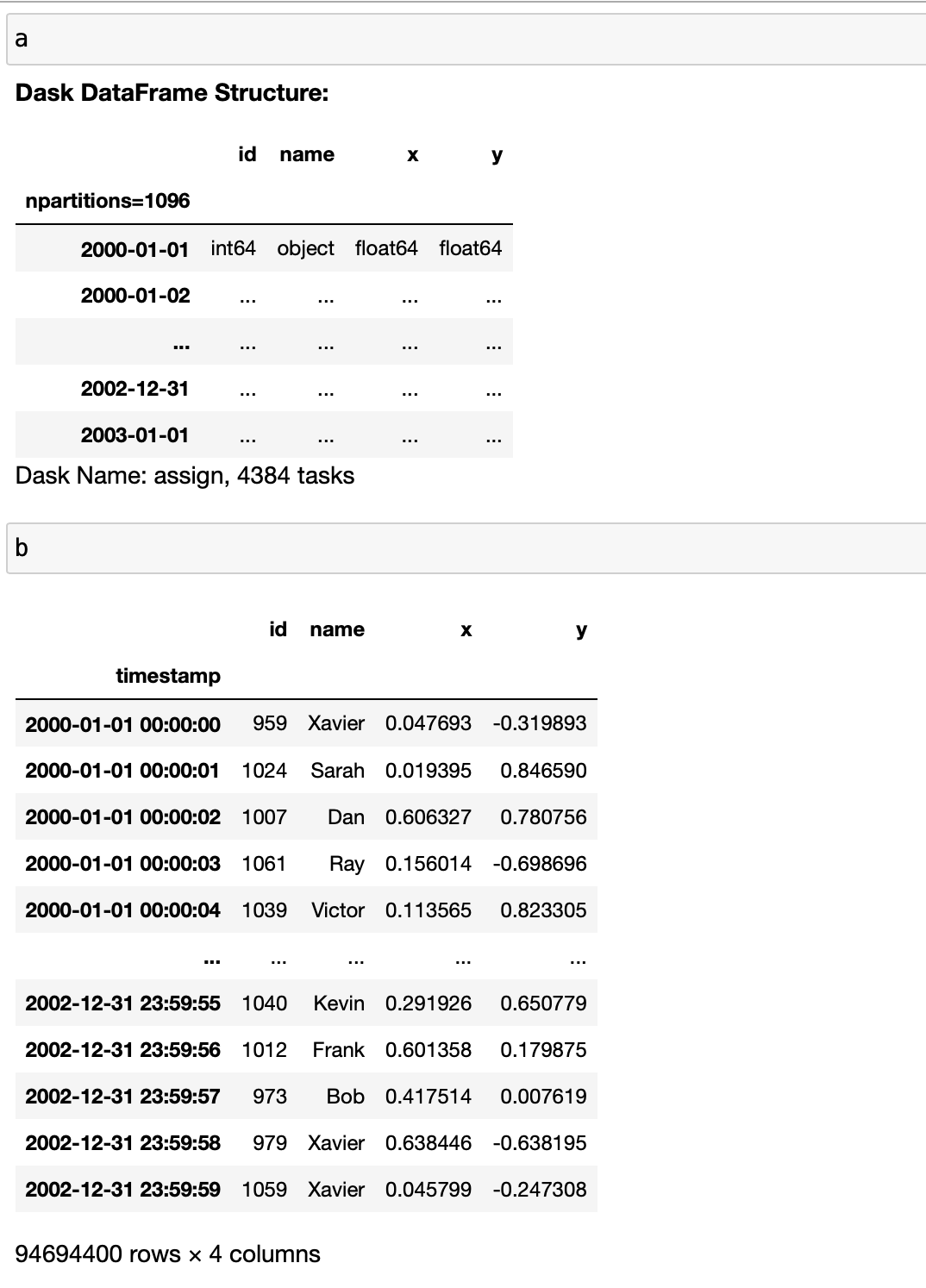
So Dask is “faster” but this isn’t really a fair comparison because Dask hasn’t actually computed our values! However, this “laziness” is what allows Dask to handle the real computations more efficiently too, and understanding this is crucial to using Dask effectively.

Understanding Dask arrays

You’re probably familiar with numpy arrays. Dask provides a high-level array collection that can help parallelize array-based workloads. This collection works with any array object that complies with the numpy array interface.

We won't cover this deeply but you should know Dask arrays exist before we dive into more low-level representations. Let's look at a basic example:

darr = ddf.to_dask_array()
darr

As with Dask dataframes, our array doesn't contain any concrete values until we call compute() on it, but we can see some relevant metadata in its string representation.

Now call compute() to see the values.

darr.compute()

And you should see output similar to that shown below.

array([[1023, 'Laura', 0.36500781383277947, 0.6642446213434765],
       [947, 'Ray', 0.9631550705255415, -0.3940023029956219],
       [966, 'Frank', 0.3825093884585072, 0.37729825767980674],
       ...,
       [951, 'Charlie', 0.18844360109998867, -0.7401836109986142],
       [925, 'Wendy', 0.6832517036766546, -0.37444048465319746],
       [1002, 'Bob', 0.05455343066171971, -0.46561159329863]],
      dtype=object)

Understanding Dask bags

Arrays and dataframes take us a long way, but you'll often want to use the parallelizing power of Dask with custom Python objects as well. Dask bags will help you here – you can put a bunch of custom objects into a Dask bag, then use Dask operations on the collection.

ddf = dask.datasets.timeseries(start="2000-01-01", end="2000-01-31", partition_freq="6d")

dbag = ddf.to_bag()
dbag
# >>> dask.bag

# only showing first 5 elements to keep it short
pprint(dbag.compute()[:5])

The output should be similar to the following:

[(1023, 'Laura', 0.36500781383277947, 0.6642446213434765),
 (947, 'Ray', 0.9631550705255415, -0.3940023029956219),
 (966, 'Frank', 0.3825093884585072, 0.37729825767980674),
 (977, 'Frank', 0.9268560208855817, -0.07482972998323256),
 (1036, 'Norbert', 0.14971748464451237, 0.2948406299270001)]

Of course, bags are more interesting when we use them with custom Python objects. We won't explore too much detail here, but you can read more about bags and see examples in the official documentation.

Other collection types

Dask has lots of collections, and you can also add third-party collections like Xarray. We’re not diving into them now but it’s important you know they exist.

Low-level representation

Now you've seen the basics of some high-level Dask functionality, let's drop down to look behind the scenes. The main concept to understand is this: a Dask dataframe is basically a collection of many smaller Pandas dataframes. If you concatenated these smaller dataframes, you would get a Pandas representation of the equivalent Dask dataframe (though in real-world cases, this is often infeasible due to memory constraints).

This image from the official documentation depicts this nicely:

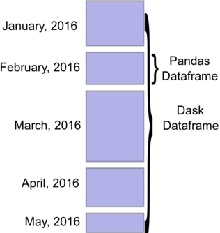
How do Dask dataframes handle Pandas dataframes?

A Dask dataframe knows only,

• How many Pandas dataframes, also known as partitions, there are;
• The column names and types of these partitions;
• How to load these partitions from disk;
• And how to create these partitions, e.g., from other collections.

Additionally, it might know the smallest and largest index value of each dataframe.

All of this information constitutes the divisions of a Dask dataframe. As long as Dask knows the metadata of these divisions – for example, knowing that each dataframe is sorted – then it can execute many operations in an optimized way.

With this additional knowledge, we can examine our dask dataframe for the data mentioned above:

ddf.npartitions
# >>> 5

pprint(ddf.divisions)

Which should show:

(Timestamp('2000-01-01 00:00:00', freq='6D'),
 Timestamp('2000-01-07 00:00:00', freq='6D'),
 Timestamp('2000-01-13 00:00:00', freq='6D'),
 Timestamp('2000-01-19 00:00:00', freq='6D'),
 Timestamp('2000-01-25 00:00:00', freq='6D'),
 Timestamp('2000-01-31 00:00:00', freq='6D'))

We can see the types with:

ddf.dtypes

Which should show:

id      int64
name    object
x       float64
y       float64
dtype:  object

And finally the columns:

ddf.columns
# >>> Index(['id', 'name', 'x', 'y'], dtype='object')

To summarize, we can see the following information about a Dask dataframe:

• The number of partitions;
• The divisions;
• The column dtypes;
• The column names.

We don't know what exactly is in the index, how many rows are in each partition, or the values. If you run:

ddf.index

You should see:

Dask Index Structure:
npartitions=5
2000-01-01    datetime64[ns]
2000-01-07               ...
                   ...      
2000-01-25               ...
2000-01-31               ...
Name: timestamp, dtype: datetime64[ns]
Dask Name: assign, 25 tasks

And try:

ddf.values

The Delayed object

The next concept for you to understand is the Delayed object. Let's start by trying to get the shape of our data. If we did this in Pandas, we’d expect to be told the number of rows and columns.

ddf.shape
# >>> (Delayed('int-919cd2bb-5fe3-4854-953e-7e95f629a591'), 4)

From the above call to shape, we see that Dask replaced the number of rows with a Delayed object. This is because Dask doesn't yet know how many rows are in our dataframe. To figure this out, it has to load each partition, call .shape[0] on the underlying dataframe, and sum up all the row numbers.

This is an expensive operation because we might have to load many files from disk, serialize them into Pandas dataframes, then call.shape on them, and finally sum up all the row counts.

Because Dask is lazy, it gives us a Delayed object. A Delayed object is an intermediate representation – it’s not yet on the lowest level as it still has methods we can call to construct new methods. As you might expect, all calls on a Delayed object are evaluated lazily.

Let's have a quick look into the Delayed object before we break it apart into the lowest-level representation.

ddf.shape[0].compute()
# >>> 2592000

Above, we call compute() on a Delayed object. This triggers the computation and gives us back the underlying Python object that it represents (which can be any Python object). We can also do other operations on a Delayed object, which will return a modified Delayed object that includes the given operation.

ddf.shape[0] // 2
# >>> Delayed('floordiv-ba9948ce982fca458e089c3aa2e4e65a')

Note how we have floordiv in the output, instead of the int that we saw before, representing the division operation that we’ve added. If we want the actual result of this operation, we still have to call compute() explicitly, as before.

(ddf.shape[0] // 2).compute()
# >>> 1296000

Why do we need Delayed objects?

Delayed objects are incredibly useful to create algorithms that can't be represented with Dask's standard user interfaces. By calling methods on Delayed objects, you are constructing a Directed Acyclic (Computation) Graph that will then be computed by Dask.

Understanding the Dask graph

We’re finally ready now to look into Dask's lowest-level representation: the Dask graph.

The Dask graph is a Directed Acyclic Graph (DAG): a graph with no cycles (including indirect or transitive cycles). Dask constructs the DAG from the Delayed objects we looked at above. We can create one and visualise it.

A Delayed object represents a lazy function call (these are the nodes of our DAG). The function call will return some data (or an object). When we pass this data into another delayed function call, we are constructing an edge to this new node. Let’s create a very simple graph:

one = dask.delayed(1, name="one")
two = dask.delayed(2, name="two")

dsum = dask.delayed(sum, name="dsum")
three = dsum([one, two])
three.compute()
# >>> 3

So we can do 1 + 2 and get the result 3. How does this work? We construct two Delayed objects:

• The first one simply holds the integer value 1;
• The second holds the integer value 2.

Next, we define a delayed sum function by wrapping Python's built-in sum.

Finally, we call sum on our delayed objects one and two. In pure Python, the code would look like this:

one = 1
two = 2

sum([one, two])
# >>> 3

This is a trivial example but it helps us understand how Dask handles things under the hood. Dask has some visualisation built in, which we can use as follows:

three.visualize()

The rectangular shapes represent data, while the circles represent operations. From this representation, Dask knows it first needs to get one and two before it executes sum.

Simple enough, right? Now let's look more deeply into Dask's internals by removing the last layer of abstraction – the Delayed object – and seeing how these graphs are saved internally.

three.dask

Dask has a high-level graph object that helps us inspect the graph. You can see that it’s grouped the three data boxes into layers for us, and also assigned them names. Now that’s nice, but we want to reach an even lower level.

Internally, a Dask graph is basically just a Python dictionary. Run:

pprint(dict(three.dask))

And you’ll see:

{'one': 1,
 'sum-eacfa1fa-4c29-451a-92e1-8f48f489c341': (,
                                              ['one', 'two']),
 'two': 2}

Now we see the graph representation in pure Python types. Let's analyze this dictionary. What we see here is a Task graph. Each task has a name that’s usually assigned automatically by a Dask higher-level interface. We can see the name of the task in the dictionary's keys.

From what we can see, the values of the dictionary are either pure data (Python objects) or some weird-looking tuple – as it is for our sum operation. Let's have a closer look at this tuple:

three.dask['sum-847f35e4-568a-42f8-8f64-c12b79b6b48e']

# >>> (, ['one', 'two'])

This tuple contains our Python function sum and two strings. This looks strange, as we’re getting back integers. But if you look closely, you’ll notice that these strings are actually task names. They represent the output of a task. In Dask:

• Values holding a single object are interpreted as data.
• Values holding a tuple are interpreted as function calls. Their arguments can hold pure data or they can reference other tasks.

So in this simple example, compute is practically:

graph = three.dask

graph['sum-eacfa1fa-4c29-451a-92e1-8f48f489c341'][0](
    [graph["one"], graph["two"]]
)

# >>> 3

Of course, the code above only works for this concrete example. It’s not parallelized so Dask does the same thing, but in a highly optimized manner. You might ask yourself how Dask knows it has to compute sum(). You can examine this by looking at the dependencies attribute of the graph. Run:

pprint(graph.dependencies)

And you’ll see:

{'one': set(),
 'sum-eacfa1fa-4c29-451a-92e1-8f48f489c341': {'one', 'two'},
 'two': set()}

Connecting DAGs to Dask dataframes

Now you understand what a DAG is and how Dask uses this low-level representation to store computation instructions, we can look into how this works on a Dask dataframe.

Let's take a look into our ddf object from before:

ddf = dask.datasets.timeseries(start="2000-01-01", end="2000-01-31", partition_freq="6d")
ddf = ddf.assign(x=ddf.x**2)
ddf.visualize()

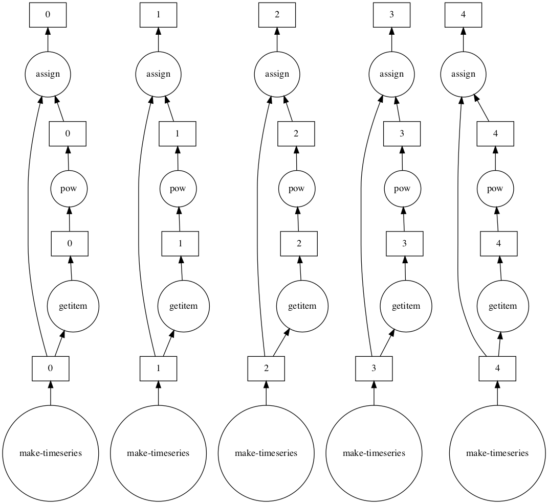
This looks slightly more complex than our previous graph but they’re actually pretty similar. Look closely and you'll notice we have several graphs – actually one per partition – that have exactly the same structure. Let's look at a single subgraph and see what it does. We have to read this graph from the bottom up.

We have:

1. make-timeseries: This is a Dask function that generates a partition of our timeseries dataframe.
2. 0,...,4: These represent our Pandas dataframe partitions.
3. Now we have two edges. Let's follow the right path as the left one has no operations:

1. getitem: We get the column x from our dataframe;
2. 0,...,4: This represents a pd.Series of our column;
3. pow: This is taking the series to the power of two;
4. 0,...,4: Data representing our series taken by the power of two.

1. Now we’re at a mergepoint. We combine the result from the previous node with the result of step 2, using an assign operation. This assigns our series to the dataframe created by step 1.
2. 0,...,4: The partitions of our end result.

If it’s your first time using Dask and not everything makes immediate sense, don't worry! This is complicated stuff, but will get more familiar. The key insight is that we can easily parallelize this operation now. We know the exact dependencies of every piece of data and each operation, so we can easily divide the work into separate processes and compute it across multiple cores.

Where is the 2?

Above, we glossed over the pow operation as “taking the series to the power of two.” But where is the 2? To find out, we'll have to dive back into the Dask graph.

ddf.dask

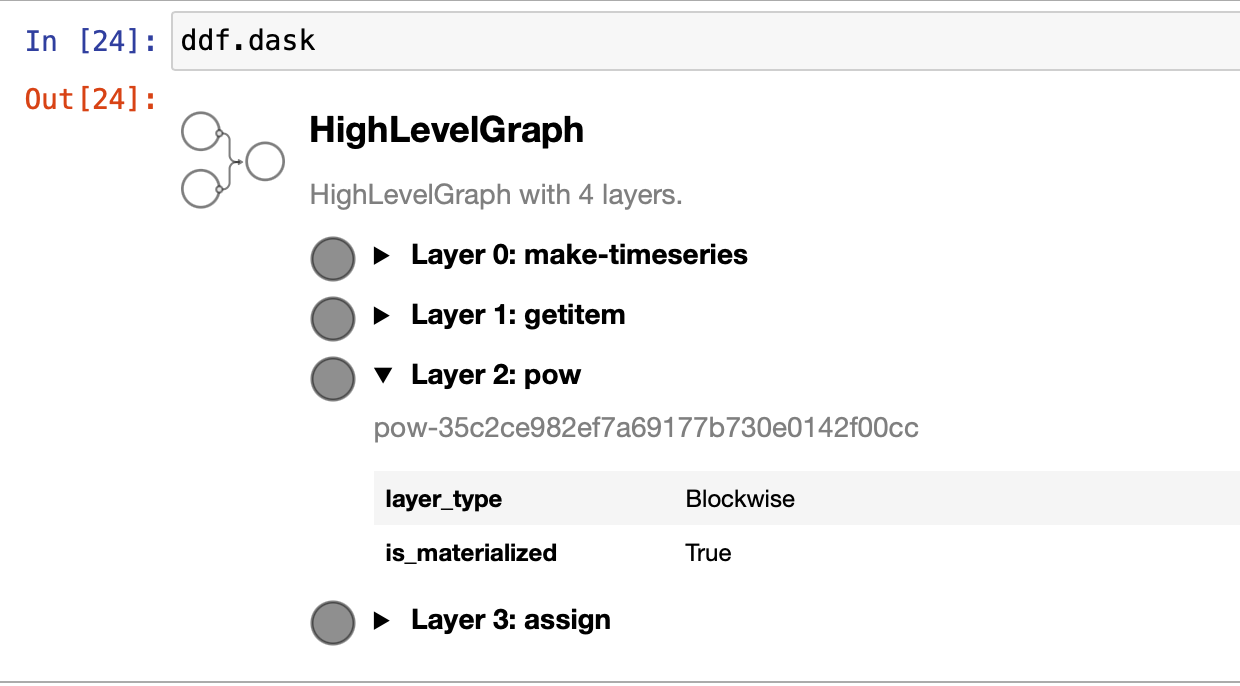
Alt text: A summary of a HighLevelGraph, showing layer 0 is make time series, layer 1 is get item, layer 2 is pow, which is expanded and layer 3 which is “assign”.

This gives us an interactive, high-level view of the layers in our graph. We still don't see the 2, so let's go deeper.

pprint(dict(ddf.dask.layers["pow-35c2ce982ef7a69177b730e0142f00cc"]))

For the above, use the long string you see after Layer 2: pow from the previous output.

You should see the full subgraph, as shown below.

{('pow-3fab3ebc9ce0a98793be54462eaaeaef', 0): (subgraph_callable-70f5782e-999c-4ccc-9eed-77221930d952,
                                               ('getitem-bba2e9806d6f82bc2b2e92ca16c51232',
                                                0),
                                               2),
 ('pow-3fab3ebc9ce0a98793be54462eaaeaef', 1): (subgraph_callable-70f5782e-999c-4ccc-9eed-77221930d952,
                                               ('getitem-bba2e9806d6f82bc2b2e92ca16c51232',
                                                1),
                                               2),
 ('pow-3fab3ebc9ce0a98793be54462eaaeaef', 2): (subgraph_callable-70f5782e-999c-4ccc-9eed-77221930d952,
                                               ('getitem-bba2e9806d6f82bc2b2e92ca16c51232',
                                                2),
                                               2),
 ('pow-3fab3ebc9ce0a98793be54462eaaeaef', 3): (subgraph_callable-70f5782e-999c-4ccc-9eed-77221930d952,
                                               ('getitem-bba2e9806d6f82bc2b2e92ca16c51232',
                                                3),
                                               2),
 ('pow-3fab3ebc9ce0a98793be54462eaaeaef', 4): (subgraph_callable-70f5782e-999c-4ccc-9eed-77221930d952,
                                               ('getitem-bba2e9806d6f82bc2b2e92ca16c51232',
                                                4),
                                               2)}

Now we see the five subgraphs, each representing a power operation. The 2 is passed in as the second value for each value.

Also, we can see how there is one task per partition. Each name is now a tuple – the first element is the layer, and the second is the partition.

If we want to pull out the function from the Dask graph, we can do that and use it just like any other Python function.

raise_to_power = ddf.dask.layers["pow-35c2ce982ef7a69177b730e0142f00cc"][('pow-35c2ce982ef7a69177b730e0142f00cc', 0)][0]
raise_to_power(2, 2)
# >>> 4
raise_to_power(2, 4)
# >>> 16

So we can see that the Dask graph contains function arguments as raw data. In our case, we used 2 as an argument, so it’s not a big deal. But we might pass entire arrays or whole data frames as arguments in many cases. This means that our Dask graphs can consume a lot of memory. The data has to be duplicated once per partition (remember, these partitions might run on different cores), making the memory use even higher.

Where next?

We've covered a lot of the internal details of the Dask graph here. Remember, you probably won't be using any of this in day-to-day usage of Dask. But these operations are very useful if you need to debug Dask code. They help your understanding of what is happening under the hood, allowing you to write more efficient Dask code.